| > | restart; |
Activation of the package
| > | with(PraSCAn); |
![]()
| > |
1st order SC network ("RC" network simulation)
Description of the circuit.
![[Maple Bitmap]](images_pracsan/prascan2.gif)
| > | SCnet:="*integration SC network *Phases Definition - Two-phase circuit |
| > | P 2 *Switch S2 between nodes 1 and 2 in even (1st) phase |
| > | S1 1 2 1 *Switch S2 between nodes 2 and 3 in odd (2nd) phase |
| > | S2 2 3 2 *Capacitor C1 between nodes 2 and 0 |
| > | C1 2 0 *Capacitor C2 between nodes 3 and 0 |
| > | C2 3 0 |
| > | .end": |
C matrix computation.
| > | CMatrixS(SCnet); |
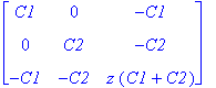
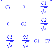
Another expression of the C matrix
| > | SetConfig(UseSqrtZ=true): |
| > | CMatrixS(SCnet); |
Definitions of the node voltages vector V=[V1e=V2e,V2e,V2o=V3o] and vector of exciting charge sources Q=[Q1e=Q2e,Q3e,Q2o=Q3o].
| > | Vectors(SCnet); |
![TABLE([0 = 0, 1 = 1, 2 = 2, 3 = 3]), TABLE([Q = Array(%id = 21395824), V = Array(%id = 21395696)])](images_pracsan/prascan5.gif)
Computation of the voltage transfer functions (VV) from input node 1 to output node 3, firstly from first (even) to first phase (Kee) and secondly from the first to the second (even) phase.
| > | Kee:=TransferS(SCnet,1,3,1,1,VV,VV); |
| > | Keo:=TransferS(SCnet,1,3,1,2,VV,VV); |
![]()
![]()
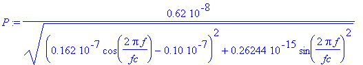
Substitution of the numerical values to the symbolic transfer function Kee and computation of the frequency response.
| > | P:=evalc(abs(subs({z=exp(I*2*Pi*f/fc),C1=6.2e-9,C2=10e-9},Kee))); |
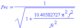
Transfer function derivated by method of equivalent resistors.
| > | Prc:=evalc(abs(subs(C1=6.2e-9,C2=10e-9,subs(R=1/fc/C1,1/(1+I*2*Pi*f*C2*R))))); |
Plot of the magnitude characteristics for both cases (charge equation method - red and method of equivalent resistors - blue).
| > | plot([subs(fc=1e4,P),subs(fc=1e4,Prc)],f=0..1000,color=[red,blue],thickness=2); |
![[Maple Plot]](images_pracsan/prascan10.gif)
The same plot but for bigger bandwidth (to the clock frequency) - demonstration of periodical frequency response of switched circuit.
| > | plot([subs(fc=1e4,P),subs(fc=1e4,Prc)],f=0..10000,color=[red,blue],thickness=2); |
![[Maple Plot]](images_pracsan/prascan11.gif)
The same plot as in the first example but for logaritmic scaling of frequency axe (magnitude in [dB]) and the same transfer function multiplied by sampled function
 .
.
| > | plots[semilogplot]([20*log10(subs(fc=1e4,P)),20*log10(subs(fc=1e4,P*sin(Pi*f/2/fc)/(Pi*f/2/fc)))],f=10..5000,thickness=2,color=[red,green]); |
![[Maple Plot]](images_pracsan/prascan13.gif)
Demonstration of tuning by the change of the clock frequency.
| > | plots[semilogplot](20*log10(subs(fc=5e4,P)),f=10..5000,thickness=2); |
![[Maple Plot]](images_pracsan/prascan14.gif)
| > |
Analysis of the Circuit with real switches
Description of the circuit with nonzero resistors of the both switches. The resistances are modeled by resistor Ron connected in series with capacitor C1.
| > | SCclr:="*real 1st order SC network |
| > | P 2 |
| > | S1 1 2 1 |
| > | S2 2 3 2 |
| > | C1 2 4 6.3e-9 |
| > | Ron 4 0 500 |
| > | C2 3 0 10e-9 |
| > | .end": |
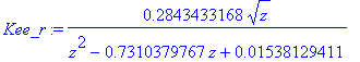
Computation of the voltage transfer function from only from first to first phase (Kee_r).
| > | Kee_r:=TransferRN(SCclr,1,3,1,1,VV,VV,1/1e5,2); |
Substitution to the
![]() and
and
![]() variables.
variables.
| > | P_r:=evalc(abs(subs({z=exp(I*2*Pi*f/fc),s=I*2*Pi*f},Kee_r))): |
Plot of the magnitude characteristics for both cases (ideal - red and real circuit - blue).
| > | plots[semilogplot]([20*log10(subs(fc=1e4,P)),20*log10(subs(fc=1e4,P_r))],f=10..1e3,color=[red,blue],thickness=2); |
![[Maple Plot]](images_pracsan/prascan18.gif)
| > |
SC Integrator
Description of the circuit.
![[Maple Bitmap]](images_pracsan/prascan19.gif)
| > | SCint:="*SC integrator |
| > | P 2 |
| > | S1 1 2 1 |
| > | S2 2 3 2 |
| > | C1 2 0 *Capacitor C2 between nodes 3 and 4 vith value 3 |
| > | C2 3 4 3 *Ideal operational amlifier - output nodes: 4, 0, input nodes: 3 and 0 |
| > | A 4 0 3 0 |
| > | .end": |
Computation of the voltage transfer functions.
| > | Kee:=TransferS(SCint,1,4,1,1,VV,VV); |
| > | Keo:=TransferN(SCint,1,4,1,2,VV,VV); |
![]()
![]()
| > |
SC Biquad in current mode with GIC
Description of the circuit.
![[Maple Bitmap]](images_pracsan/prascan22.gif)
| > | SCbiq:="*SC Filter with GIC P 2 C1 1 0 C2 1 6 C3 5 0 C4 5 6 Ck1 8 9 Ck2 2 3 1 Ck3 10 11 Ck4 4 5 1 CL 7 0 S1 1 7 1 S2 7 0 2 S3 1 8 2 S4 2 9 2 S5 8 0 1 S6 9 0 1 S7 3 10 1 S8 4 11 1 S9 10 0 2 S10 11 0 2 A1 1 3 4 0 A2 5 3 2 0 .end": |
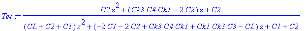
Computation of the current transfer function from input node 1 to output node 6 and from first to te first phase.
| > | Tee:=TransferS(SCbiq,1,6,1,1,QQ,QQ); |
![]()
![]()
Computation of the the same transfer function, but now with respect to entered numerical values of capacitors Ck1 and Ck4 (function TransferN is used).
| > | Tee:=collect(TransferN(SCbiq,1,6,1,1,QQ,QQ),z); |
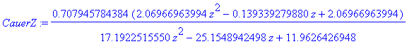
Entering transfer function of a filter with Cauer approximation of magnitude characteristic in Z domain.
| > | CauerZ:=0.707945784384*(2.06966963994*z^2-0.139339279880*z+2.06966963994)/(17.1922515550*z^2-25.1548942498*z+11.9626426948); |
Comparison of coefficients of both transfer functions (calculated and required) - assembling of equations.
| > | eq_num:=coeff(numer(Tee),z,1)/(coeff(numer(Tee),z,2))=coeff(numer(CauerZ),z,1)/(coeff(numer(CauerZ),z,2)); |
| > | eq_den:=seq(coeff(denom(Tee),z,i)/(coeff(numer(Tee),z,2))=coeff(denom(CauerZ),z,i)/(coeff(numer(CauerZ),z,2)),i=0..2); |
![]()
![]()
Solving of the equations for normalized clock period - finding (normalized) values of all cappacitors to both transfer function be equal.
| > | T:=2*Pi/10: |
| > | sol:=solve({eq_num,eq_den,Ck1=T,Ck3=T,CL=T}):solf:=evalf(sol,4); |
![]()
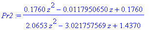
Substitution of capacitor calculated values.
| > | Pr2:=subs(solf,Tee); |
Calculating of magnitude characteristic of resulted transfer function and its plot.
| > | Prp:=subs(z=exp(s*T),Pr2):Prp_m:=evalc(abs(subs(s=I*omega,Prp))): |
| > | plot(20*log10(Prp_m),omega=0..5,thickness=2); |
![[Maple Plot]](images_pracsan/prascan31.gif)
| > |
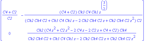
Twoport parameters calculation
Two phases -> fourport parameters, admitance and csascade.
| > | TwoNPortS(SCbiq,1,6,Y11); |
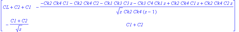
| > | TwoNPortS(SCbiq,1,6,Y); |
![]()
![]()
![]()
![]()
| > | TwoNPortS(SCbiq,1,6,A11); |
| > |
| > |
General SC biquad - real analysis
Circuit diagram.
![[Maple Bitmap]](images_pracsan/prascan38.gif)
Subcircuit definition - ideal switch
| > | switch_ideal:=" |
| > | .subckt SP n1 n2 p1 |
| > | S1 n1 n2 p1 |
| > | .ends |
| > | .end": |
Subcircuit definition - switch with nonzero Ron
| > | switch_res:=" |
| > | .subckt SP n1 n2 p1 |
| > | S1 n1 n3 p1 |
| > | R1 n2 n3 Ron |
| > | .ends |
| > | .end": |
Description of the circuit - biquadratic section as a bandpass filter.
| > | cir:=" |
| > | P 2 |
| > | C1 5 6 1 |
| > | C2 7 9 1 |
| > | C3 4 8 5806/10000 |
| > | C4 2 3 1 |
| > | C5 2 9 175/10000 |
| > | C6 1 7 175/20000 |
| > | C7 1 2 175/10000 |
| > | C8 10 0 1 |
| > | XS1 4 0 2 SP |
| > | XS2 4 2 1 SP |
| > | XS3 3 5 2 SP |
| > | XS4 5 0 1 SP |
| > | XS5 6 0 2 SP |
| > | XS6 6 7 1 SP |
| > | XS7 8 0 2 SP |
| > | XS8 8 9 1 SP |
| > | XS9 11 10 1 SP |
| > | A1 3 0 0 2 |
| > | A2 9 0 0 7 |
| > | A3 1 0 10 1 |
| > | .include cirs |
| > | .end": |
| > |
Analisis of the ideal circuit
Consider ideal switched.
| > | cirs:=switch_ideal: |
Computation of symbolic transfer function.
| > | collect(TransferS(cir,11,9,1,1,VV,VV),z); |
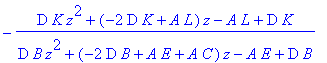
| > | eval(%,[C1=A,C2=B,C3=C,C4=D,C5=E,C6=K,C7=L]); |
Computation of numeric transfer function, magnitude and phase frequency response.
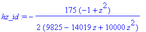
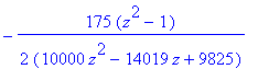
| > | hz_id:=TransferN(cir,11,9,1,1,VV,VV); |
| > | MH:=MagnitudeHz(evalf(hz_id)); |
| > | PH:=PhaseHz(-evalf(hz_id)): |
![]()
Using function for real transfer calculation (in this sace must return the same result).
| > | normal(TransferRN(cir,11,9,1,2,VV,VV,1,2)*z); |

Plot of the characteristics.
| > | plot(MH(omega),omega=0.5..1.1,thickness=2); |
| > | plot(PH(omega),omega=0.5..1.1,thickness=2); |
![[Maple Plot]](images_pracsan/prascan44.gif)
![[Maple Plot]](images_pracsan/prascan45.gif)
| > |
Analisis of the real circuit
Setting

![]() and computation of real transfer funftion of the circuit.
and computation of real transfer funftion of the circuit.
| > | Ron:=1/100; |
| > | cirs:=switch_res: |
| > | hz_re1:=evalf(TransferRN(cir,11,9,1,2,VV,VV,1,2)*z); |
![]()
The transfer function is near the same as the transfer function of ideal circuit.
| > | hz_id; |
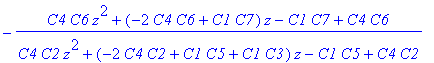
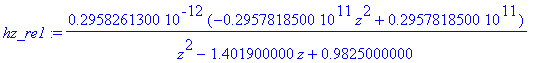
| > | simplify(evalf(numer(hz_re1),9)/denom(hz_re1)-hz_id); |
![]()
Ccomputation of real transfer funftion for different values of Ron.
| > | Ron:=1/25; |
| > | hz_re2:=evalf(TransferRN(cir,11,9,1,2,VV,VV,1,2)*z); |
| > | Ron:=1/20; |
| > | hz_re3:=evalf(TransferRN(cir,11,9,1,2,VV,VV,1,2)*z); |
| > | Ron:=1/10; |
| > | hz_re4:=evalf(TransferRN(cir,11,9,1,2,VV,VV,1,2)*z); |
![]()

![]()

![]()

Computation of transfer pole magnitudes for all cases.
| > | map(abs,[solve(denom(hz_re1))]); |
| > | map(abs,[solve(denom(hz_re2))]); |
| > | map(abs,[solve(denom(hz_re3))]); |
| > | map(abs,[solve(denom(hz_re4))]); |
![]()
Poles are outside unit circle in the last case (for

![]() ) - circuit is unstable.
) - circuit is unstable.
| > | map(abs,[solve(denom(hz_re4))]); |
![]()
Comparison of the magnitude responses for various switch Ron values.
| > | plot([MagnitudeHz(hz_re1)(omega),MagnitudeHz(hz_re2)(omega),MagnitudeHz(hz_re3)(omega)],omega=0.5..1.1,color=[red,green,blue],legend=["Ron=1/100","Ron=1/25","Ron=1/20"],thickness=2); |
![[Maple Plot]](images_pracsan/prascan62.gif)
| > |
SI integrator
Description of the circuit.
![[Maple Bitmap]](images_pracsan/prascan63.gif)
| > | SIint:="*SI integrator |
| > | P 2 |
| > | *basic memory cells T1, T2 and T3 |
| > | T1 1 1 2 1 |
| > | T2 1 1 1 1 |
| > | T3 2 1 1 alpha |
| > | *output conductance of the cells T1 and T2 - lossy integrator |
| > | *G12 1 0 1 0 2*G |
| > | *output conductance of the cell T3 |
| > | *G3 2 0 2 0 G3 |
| > | .end": |
Modeling of the output conductance by means of a voltage controlled current source.
![[Maple Bitmap]](images_pracsan/prascan64.gif)
Compilation of circuit admitance matrix.
| > | CMatrixN(SIint); |
Computation of the current transfer function from first to first phase.
| > | Kee:=TransferN(SIint,1,2,1,1,QQ,QQ); |
![]()
Ideal analysis (ideal switches - circuit withouth transient performance)!!!
| > |
SI circuit with switched
Description of the circuit.
![[Maple Bitmap]](images_pracsan/prascan67.gif)
| > | SIgm:="*SRO_RLC with switched transkonductances |
| > | P 2 |
| > | T1 1 1 2 1 |
| > | T2 1 1 1 1 |
| > | T3 2 1 1 alpha1 |
| > | T4 3 1 1 alpha1 |
| > | T5 5 1 1 alpha2 |
| > | S1 2 0 2 |
| > | S3 1 5 1 |
| > | S4 5 0 2 |
| > | G6 3 0 3 0 1 |
| > | G7 4 0 3 0 1 |
| > | S2 4 0 2 |
| > | G1 0 1 2 4 gm1 |
| > | T8 6 6 1 1 |
| > | T9 7 7 2 1 |
| > | T10 4 7 2 alpha3 |
| > | T11 4 6 1 alpha3 |
| > | S5 6 7 2 |
| > | S6 7 0 1 |
| > | G2 0 6 4 0 gm2 |
| > | .end": |
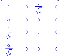
Computation of the circuit input impedance in node 2 in second (even) phase.
| > | Zin:=TransferN(SIgm,2,2,1,1,QQ,VV); |

Transformation of the input impedance from z domain to s domain by means of inverse backward Euler trasformation (BD).
| > | Zin_p:=normal(subs(z=1/(1-s),Zin)); |
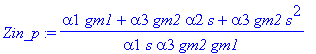
The input impedance corresponds to impedance of the RLC series resonant circuit.
| > | expand(Zin_p); |
![]()
Computation of the voltage transfer function from node 2 to node 4 both in even phase (EE).
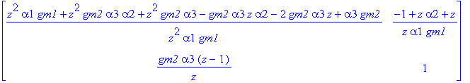
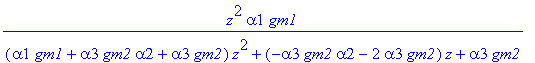
| > | Tee:=collect(TransferN(SIgm,2,4,1,1,VV,VV),z); |
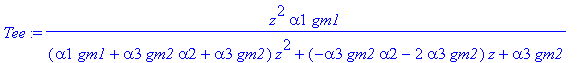
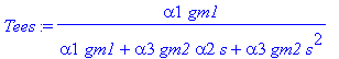
Transformation of the transfer function from z domain to s domain by means of inverse backward Euler trasformation.
| > | Tees:=normal(subs(z=1/(1-s),Tee)); |
Computation of the impedance Z11 parameter of the circuit.
| > | TwoNPortN(SIgm,2,4,Z11); |

Computation of the four-port chain matrix of the circuit.
| > | TwoNPortN(SIgm,2,4,A); |
| > | collect(1/%[1,1],z); |
| > |